Start tracking
Before tracking, first make sure to calibrate stage-camera Getting Started. This only need to be done once when the light path is modified. Then simply click on the Tracking checkbox on the bottom right corner of the GUI. A short instructional dialog will appear. Then click on the part of an animal where you would like to be the center of tracking. The animal is now being tracked.
The tracking algorithm
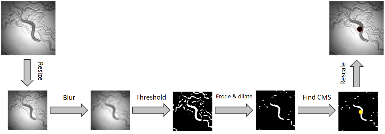
To effectively track the worm, ensuring it remains centered in the image, we must adjust the stage to compensate for the worm's movement. This involves comparing the worm's current position with its previous one and using the displacement to relocate the stage accordingly.
Resizing
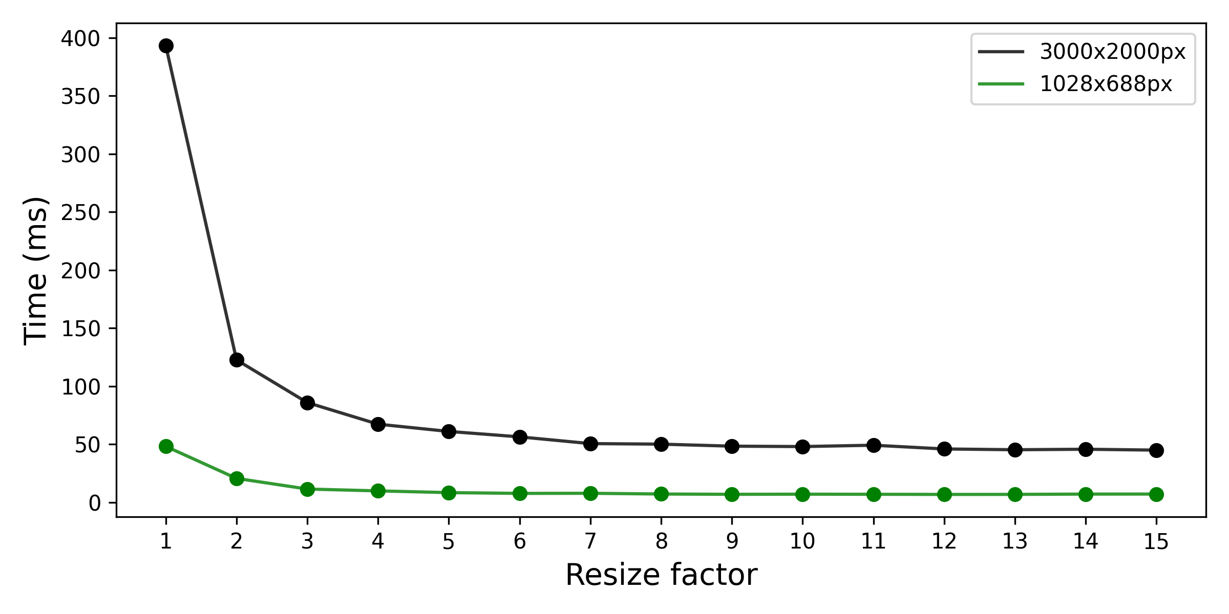
The initial step involves resizing the image to a smaller dimension, a crucial measure aimed at reducing computational load. This optimization significantly accelerates the tracking algorithm, enabling a higher frame rate.
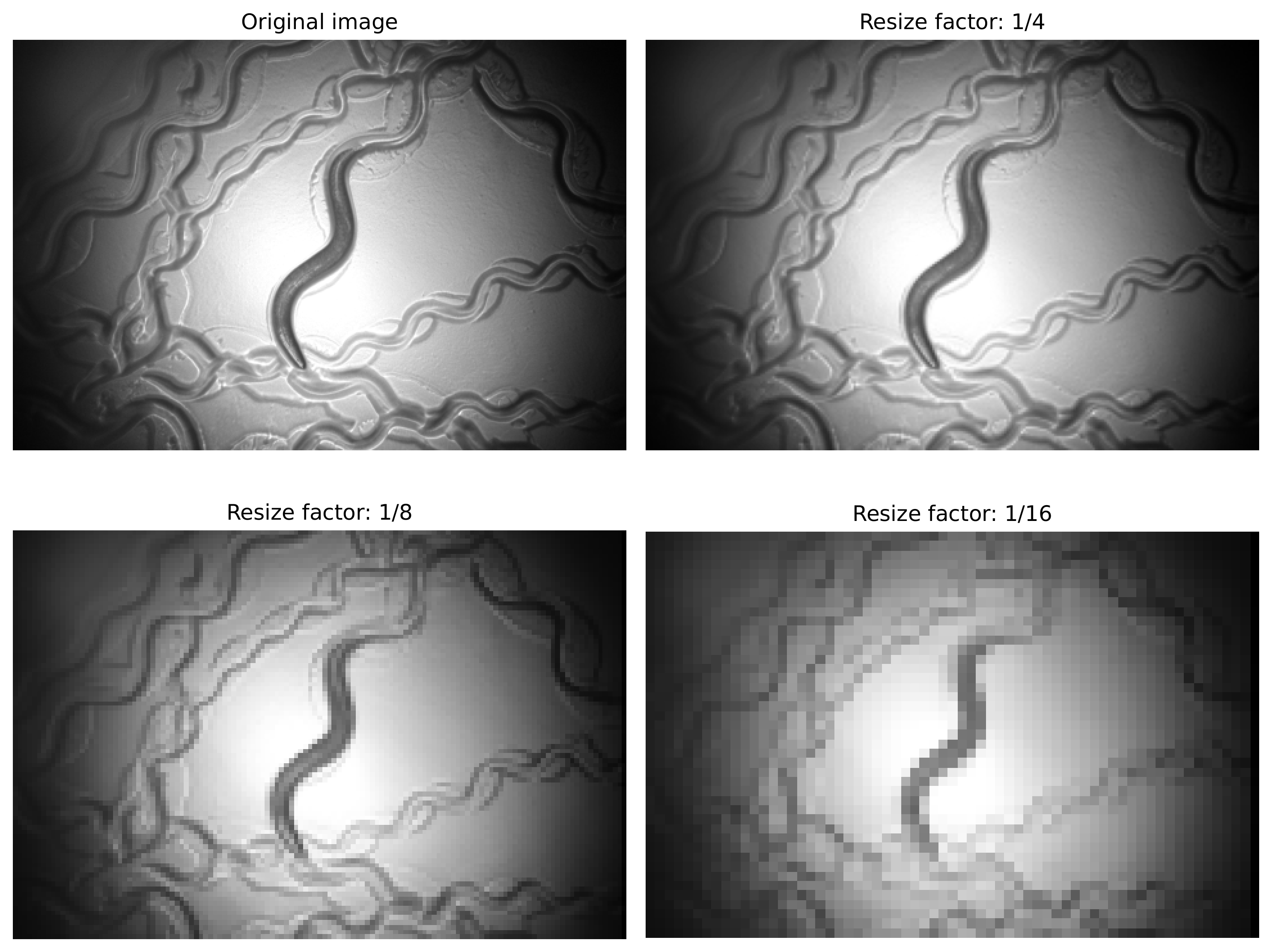
Depending on the resizing method employed —such as the cv2.resize() for a basic resizing technique— there might be a necessity to apply a blur to the image before resizing. This blurring process aims to mitigate the potential aliasing effect that could arise during downsampling. Further details on the aliasing effect can be found here.
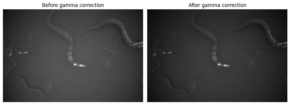
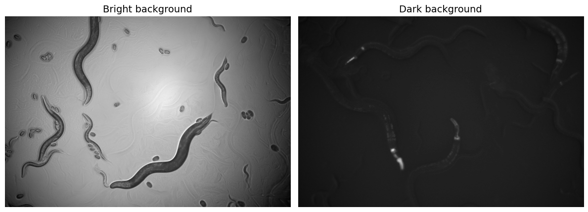
It is worth noting that, while working with the dark background recordings, we apply a gamma correction to the image before resizing. This correction aims to enhance the worm's contrast, making it easier to track.
Blurring
The next step involves applying a blur to the image. It makes the image appear smoother, which is a desirable effect as it reduces the noise in the image. More specifically, it reduces the high-frequency components of the image and preserves the low-frequency components. The blur is applied to the image using the cv2.GaussianBlur() function, which applies a Gaussian kernel to the image. The larger the kernel size, the more blur is applied to the image.
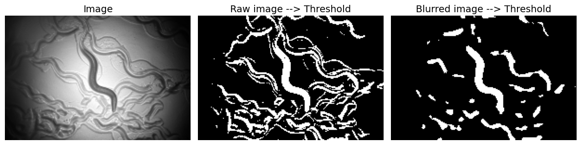
Thresholding
To find the center of mass (CMS), it is required to work with a binary image - an image with only two possible values for each pixel. To do so, we apply a threshold to the image, which converts the image to a binary image. Simply said, for dark background images, the thresholding process involves converting the image to grayscale and then setting all pixels with a value above a certain threshold to white (foreground) and all pixels below the threshold to black (background). Depending on the type of recording, whether the background is dark and the worm is bright or vice versa, we apply a different thresholding method. We use the skimage.filters.threshold_yen() method and the cv2.adaptiveThreshold() method to apply the thresholding to the dark and bright background recordings, respectively.
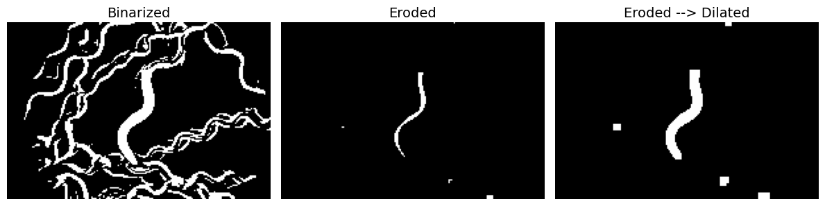
Erosion & Dilation
The next step involves applying an erosion and dilation filter to the image. The erosion filter removes small white spots from the image, whereas the dilation filter fills in small holes in the image. By having erosion followed by dilation, we can remove small white spots while preserving the worm's shape. We can apply them for several iterations based on how noisy is the image, how many objects are in the image, how close the objects are to each other, etc. However, having strict erosions and dilations can lead to the loss of the worm or the merging of different objects into one.
Finding the center of mass (CMS)
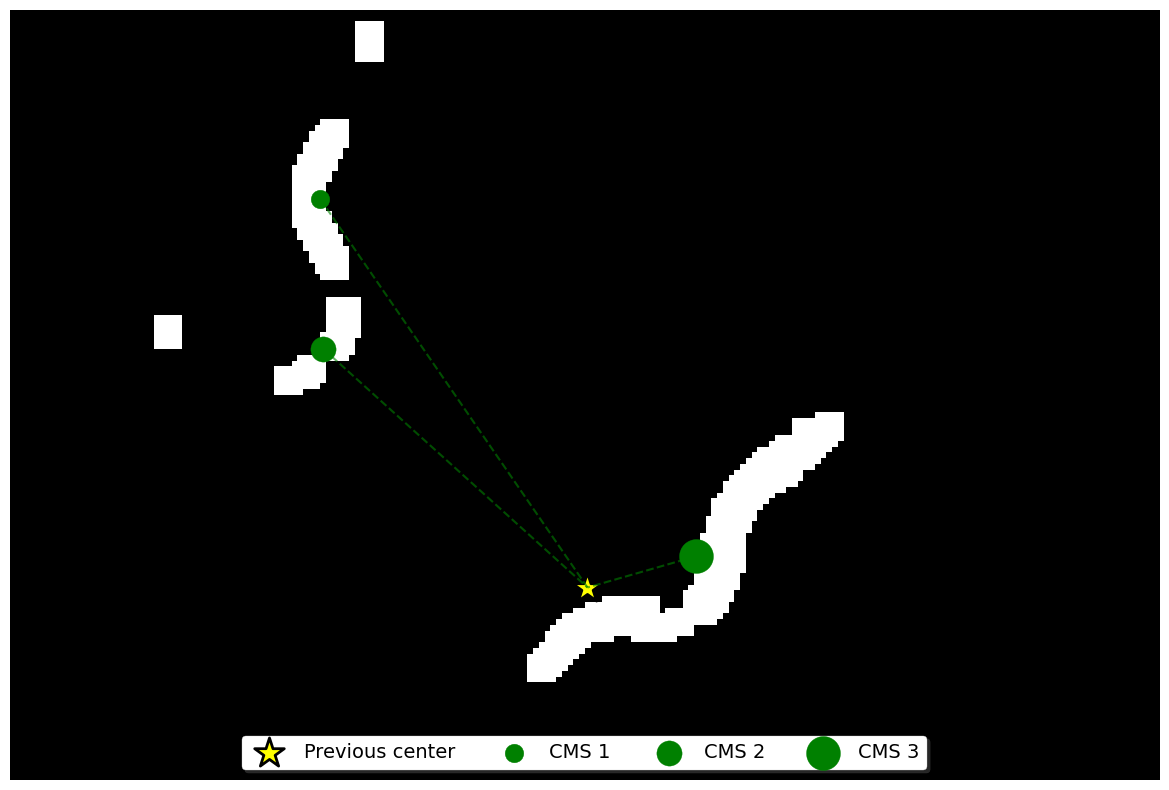
The final step involves finding the center of mass (CMS) of the worm. By having a binary image, we can find the CMS locally for each white region (plausible worm) in the image. To do so we use the skimage.measure.regionprops_table(<BINARY_IMG>, properties=('centroid', 'area')) method, which returns the CMS and the area of each white region in the image. We then keep the top K regions with the largest area.
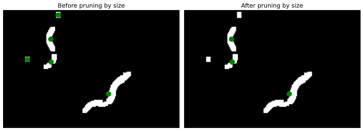
Then we compute the Euclidean distance (a.k.a. L2 norm) between the previous frame's final CMS and the current frame's CMS for each region. Because of the high frame rate, the worm's movement between two consecutive frames is expected to be small. Therefore, we can assume that the region with the smallest distance is the worm. Please note that, using this approach, we are enable to track a worm even if there are multiple worms in the field of view.
Finally, we can use the CMS of the worm and compute the displacement between the CMS and the center of the image. This displacement is up-scaled and then used to move the stage accordingly. In other words, we move the stage such that the worm is centered in the image throughout the recording.
We also show that as far as there is a good contrast between the worm and the background, the tracking algorithm is robust to the lighting conditions.
Discussion
Due to the above explanations, this tracking procedure does not guaranteed to maintain it’s course on the same animal if the animal is occluded or overlaped with other animals because it does not have a conceptual data of what an animal is, and rather treated eveything equally as intensities on an image. This problem can be mitigated by: reducing the tracking radius, changing the intensity range, reducing population density, or performing the experiment in dual-color mode